Poincaré sections are a tool for understanding chaos in dynamical systems. Here is an interactive one for the double pendulum (best enjoyed on desktop). Click in the main pane below to add an orbit. Click here for a tour. Details about what it all means are below.

What is a Poincaré section?

Understanding a dynamical system is hard, especially when there are a lot of degrees of freedom. We usually think of the state of a system as a point in a high-dimensional space. For the double pendulum in a plane, it’s four dimensional. I don’t know about you, but I can’t visualize a point moving around in 4 dimensions, and the double pendulum is one of the easier systems!

Enter the Poincaré section. Henri Poincaré (who touched so many parts of physics and math) came up with this nice tool. Pick a lower-dimensional slice (say a 2-dimensional surface) of your space that is intersected by the motion of points in this space. Now pick a point on that surface. Follow the motion of that point until it hits your slice again, then put a dot there (going from the first point on the slice to the second is called the Poincaré map). Now just keep going! The Poincaré section will be able to show you different behaviors – (quasi)periodic orbits, resonances, and chaos. Here’s an example you can play with to help get the idea:

We’re watching dynamics on the surface of a torus, with different frequencies for the two directions (“longitude” and “latitude”). This type of system only has periodic orbits, some them being resonant.

What to look for

Try to click around in the interactive Poincaré section at the top of the page to find these phenomena for yourself:

(Quasi)periodic orbits

Like on the torus above, a quasiperiodic orbit is restricted to intersecting a very small part of the plane. It can’t fill a volume. Most quasiperiodic orbits will have irrational frequency ratios, and they will end up tracing out a curve on the plane. There can be many such orbits nested inside each other:

At low energies, the double pendulum is chock full of quasiperiodic orbits with irrational frequency ratios. (In an integrable system, the phase space is basically made up of a bunch of nested tori with different frequency ratios; then the Poincaré section will look like the kinda boring picture here, just a bunch of nested curves).

Resonances

If the frequency ratio happens to be rational, then the Poincaré map will recur. That is, every nth dot you put on the Poincaré section will be in the exact same spot. The number n is called the order of the resonance. Try this above, by setting the torus’s frequency ratio to something like 3/2=1.5, or 4/3≅1.333. Here’s an example in the double pendulum:

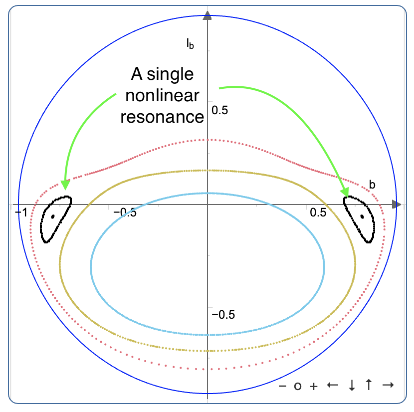
Nonlinear resonances

Suppose we’re close to an exactly resonant orbit of order n. Nearby, we might find nonlinear resonances. These are quasiperiodic orbits with irrational frequencies, but they almost-recur every nth time they hit the section. They trace out little loops around the resonances, hitting each of the n little loops once before returning to the first one.

Chaos

A chaotic orbit doesn’t recur or trace out a curve. Quite the opposite – it explores a whole volume! We only get to plot a finite number of points on the Poincaré section, so a chaotic trajectory ends up looking like dust that’s filling an area.

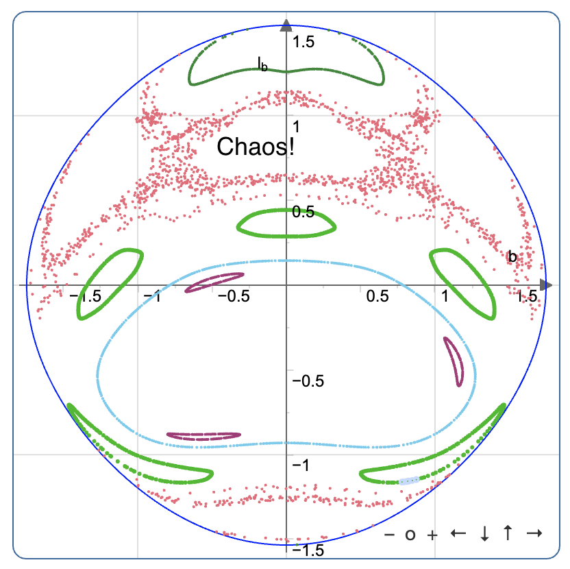
Here we can see a single chaotic orbit trying to fill out an area of the Poincaré section. Nearby there are ordinary quasiperiodic trajectories (light blue) and nonlinear resonances (shown: ones with orders 3 (purple) and 5 (green)). One really cool thing about dynamical systems is that their phase space can have chaotic regions and quasiperiodic regions coexisting in harmony right next to each other.

Islands on islands: fractal behavior

What’s this: an ordinary quasiperiodic orbit (green), surrounded by nonlinear resonances (red and blue)? Zoom out!

That green loop in the middle was itself part of a nonlinear resonance, with order 5. When zoomed in, the red loops looked like they have order 5, and the blue loops like they have order 8. But when you zoom out, you see all red loops are part of the same orbit. That orbit has to visit each of the 25=5×5 loops once before returning to the first loop. Similarly, the blue trajectory has to visit 40=5×8 islands before returning to the first one!

The fact that you can find islands around islands (around islands…) is a hallmark of fractal behavior.

If you click around, you find that these are islands of regularity in a sea of chaos:

Homoclinic orbits

Close to where islands appear, you can find something called a hyperbolic fixed point – these look like an “X”, where flows on opposite sides of the X have to move in opposite directions. Associated to these points, we can have an orbit that gets arbitrarily close to (but never reaches) the fixed point, if we go far enough forward or backward in time. Two opposite legs of the X are repelling from the fixed point, and two are attracting.

It’s possible for a trajectory to be attracted to the fixed point going into the future, and repelled from that same fixed point far in the past. This kind of trajectory is called a homoclinic orbit. Here’s the closest to one that I could get in the double pendulum:

Homoclinic orbits are important in understanding the transition to chaos.

The double pendulum’s math

One of the simplest dynamical systems that displays all these rich phenomena is the double pendulum.

It has a four-dimensional phase space: the two angles $(\alpha, \beta)$, and their conjugate momenta $(l_\alpha, l_\beta)$. The Hamiltonian for a scaled version of this system is

You can work out the four equations of motion from Hamilton’s equations. For any phase space variable $\xi$, its time derivative comes from the Poisson bracket with the Hamiltonian.

With the canonical Poisson brackets $\{\alpha, l_\alpha\}=1 = \{\beta,l_\beta\}$ and all others vanishing, Hamilton’s equations are

They are some not very pretty nonlinear equations that I will not repeat here, but your computer doesn’t mind.

We are making Poincaré sections for exactly this system at the top of the page. The surface that we’re cutting through is at constant energy $H=E$, where you choose the energy with a slider. Then further intersect with $\alpha=0$, only plotting points that cross through in the positive $\alpha$ direction, i.e. $d\alpha/dt > 0$. That corresponds to the upper arm of the pendulum being instantaneously vertical (at the bottom of its motion), and rotating in the counter-clockwise direction. The two variables that are being plotted are $(\beta, l_\beta)$ on the horizontal and vertical.

Limitations

Some of these limitations are identical to what’s on the Kerr spherical photon orbit page.

• The major limitation is that this is in javascript, which is not ideal for numerical work. There are very few numerical libraries.
• JSXGraph is really not designed for putting tens/hundreds of thousands of points onto plots – their points have many features I don’t need.
• JSXGraph only has fixed-step-size integrators, no adaptive ones. I picked what seemed like a reasonable step size in most of parameter space.
• The numerical integrator from JSXGraph that I use is a fixed step-size RK4 integrator. RK4 has no energy-error guarantee, so it is poorly suited to generate Poincaré sections. Energy drift and other integration errors will smear out fine details, and worse yet will even connect quasiperiodic orbits to chaotic ones.

Acknowledgments

This toy makes use of JSXGraph. The ‘tour’ uses intro.js. The torus demo uses three.js and threestrap. It was originally inspired by some of the coursework in Jack Wisdom’s dynamics class at MIT. I started coding this up when I was teaching a grad dynamics class in 2018. Thanks to Jenny, Nic, and Niels for editorial feedback and beta testing. Thanks to Niels for UI feedback.

Suggestions welcome! Or fork the code for this web site and send a PR :)