These notes are intended for students (or profs) aware of the multipole expansion for electrostatics in terms of symmetric tracefree (STF) tensors. Standard texts on electrodynamics (like Jackson) hardly mention the STF version, though it is extremely well-known to researchers in GR.

Update 2025-06-17: I am updating these notes because of two issues. First, Alan Guth pointed out to me, I missed terms that were pure gauge (I incorrectly claimed they vanished). Second, Cyril Pitrou pointed out to me this lovely paper by Damour and Iyer (1991) which does the whole dynamical case (i.e. the radiative multipole expansion), and pointed out that I had a factor which is only correct in the dipole case. Therefore I am cleaning up my error and reworking some of the discussion.

Refresher: Electrostatic STF multipole expansion

Before getting to magnetostatics, we’ll start with electrostatics. This is easier since we only need to solve for the scalar potential, which satisfies

We’re interested in the case where $\rho$ vanishes outside of a compact region. The most efficient way to get to the STF version of the multipole expansion is to start from the Green’s function solution,

We then take the function $1/|\bs{x}-\bs{x}'|$ and perform a multivariate Taylor series expansion about the point $\bs{x}'=0$, since far away from the source, $|\bs{x}'| \ll |\bs{x}|$. This expansion is

In the $\ell$ index tensor $\pd_{j_1} \pd_{j_2} \cdots \pd_{j_\ell} (1/r)$, all indices are obviously symmetric; they are also tracefree away from the origin, where we get a delta function, owing to $\cd^2 (1/r) = -4\pi \delta_{(3)}(\bs{x})$. Since this tensor is symmetric and tracefree (STF), we are free to take only the STF part of the product of $\bs{x}'$ direction vectors. We denote this with angle brackets around the relevant indices,

Plugging this in to the Green’s function integral, we get

where we have defined the $\ell$th STF multipole tensor of the source as

For example, the $\ell=0$ case is just the total charge $Q = \int \rho(\bs{x}) \ d^{3} \bs{x}$; the $\ell=1$ case is the charge dipole $p^i=Q^i=\int \rho(\bs{x}) x^i \ d^{3} \bs{x}$, and so on.

Magnetostatic multipole expansion

We can apply our results from the electrostatic multipole expansion to magnetostatics, using the potential formulation. In magnetostatics, we are trying to find a magnetic field $\bs{B}(\bs{x})$ satisfying

where as usual $\cd\cdot\bs{B}=0$, and in statics, conservation of charge demands that $\cd\cdot\bs{J}=0$. Now we go to the potential formulation, $\bs{B}=\cd\times\bs{A}$, and use our gauge freedom to go to Coulomb gauge, $\cd\cdot\bs{A}=0$. Plugging in, we are now trying to solve

In Cartesian coordinates, this is just three independent copies of the Poisson equation, one for each Cartesian component $A^{i}$. Therefore we can use the Green’s function for the scalar Laplacian’s for each component,

Just like in the electrostatic case, we Taylor expand $\tfrac{1}{|\bs{x}-\bs{x}'|}$, pull things out of the integrals, etc. Essentially, we are just making a replacement in the electrostatic case: $\Phi \to A^{i}, \tfrac{\rho}{\epsilon_{0}} \to \mu_{0} J^{i}$. This means our multipole moments get an extra index that does not participate in the STF operation. As it stands, our solution is

where we defined some moment integrals

which are STF only on the $j_{1}\cdots j_{\ell}$ indices after the semicolon.

Notice that the $\ell=0$ term vanishes – no magnetic monopoles! – by conservation of charge. Integrate $(\cd\cdot\bs{J})x^{j}$ and use integration by parts:

The left hand side vanishes since in magnetostatics, $\cd\cdot\bs{J}=0$. Therefore the $\ell=0$ magnetic monopole moment vanishes, $G^{i}=0$. [As an exercise, try a similar approach with $\int (\pd_i J^i) x^{j_{1}}x^{j_{2}}\cdots x^{j_{\ell}} \ d^{3}\bs{x}$, and see if you can generate an identity for arbitrary $\ell$.]

Before handling the arbitrary $\ell$ term, let’s write the dipole in the traditional form seen in e.g. Griffiths. The traditional form for a magnetic dipole is

Here the magnetic dipole pseudo-vector is related to the 2-index magnetic dipole tensor,

This gives the ideal dipole magnetic field

except that we have dropped a singular $\mu_{0}m^{i}\delta_{(3)}(\bs{x})$ term.

Aside on Young tableau and STF decomposition

It seems like we’ve discarded some information — only the antisymmetric part of $G^{i;j}$ contributed to $m^{i}$. What about the symmetric part? It turns out nothing has been lost.

The next step for understanding these magnetic multipole tensors requires a little knowledge of how Young diagrams classify the index symmetries of tensors (ok, maybe not strictly necessary, but this was how I first realized what to do). We know that the tensor $x^{\langle j_{1}}x^{j_{2}}\cdots x^{j_{\ell}\rangle}$ lives in the representation labeled by the diagram of shape $(\ell)$,

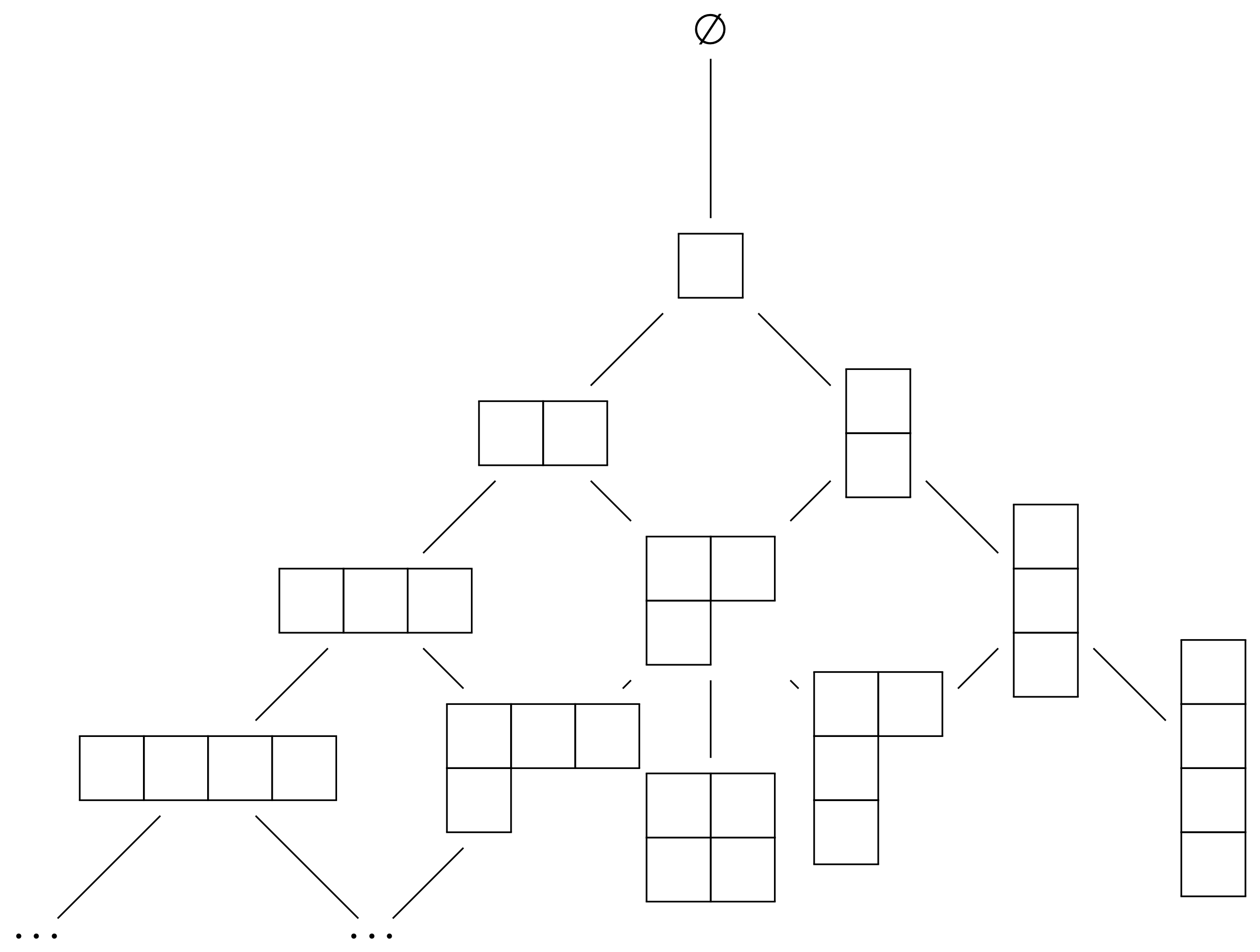
Now recall that when we tensor-product a vector with some tensor in a diagram with shape $\lambda$, we generate tensors in irreps related by adding one box at the end of any allowed row or as a new row underneath (the decomposition of tensor products into irreps is determined by the Littlewood–Richardson rule; adding one box where allowed is the simplest case. This is encapsulated in a Hasse diagram called Young’s lattice, which gives a partial order on Young diagrams, seen in here:

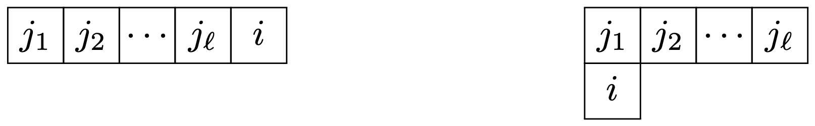
Now, since $x^{\langle j_{1}}x^{j_{2}}\cdots x^{j_{\ell}\rangle}$ lives in the $(\ell)$ representation, we know that tensoring with $J^{i}$ can produce content in exactly two representations: the $(\ell+1)$ diagram, and the $(\ell,1)$ diagram, having shapes

These above statements were for Young tableaux labeling the representations of GL(3). Once we introduce our metric $\delta_{ij}$ and go to SO(3), we can do a further trace decomposition. At the same time we’ve also introduced the Levi-Civita tensor $\epsilon_{ijk}$, which lives in the irrep labeled by 3 boxes stacked vertically. We can use the Levi-Civita tensor to dualize $p$ antisymmetric indices to $3-p$ indices, which is how we replaced $G^{i;j}$ with $m^i$. The ultimate goal is to decompose arbitrary tensors into combinations of STF tensors, $\delta_{ij}$, and $\epsilon_{ijk}$.

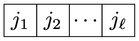
To do this we can use a rule from Blanchet and Damour (1986) which is also in Damour and Iyer (1991). You can build the decomposition inductively starting from the tensor product of just a single vector with an $\ell$-index STF tensor (here we use STF multindex notation)

where everything with a hat is STF, and the three pieces on the RHS are

This is akin to $\boldsymbol{1}\otimes \boldsymbol{\ell} = (\boldsymbol{\ell - 1}) \oplus \boldsymbol{\ell} \oplus (\boldsymbol{\ell+1})$ in angular momentum coupling. Let me comment here: Blanchet and Damour say that this expression (which is their (A3)) is “straightforwardly checked.” I did check it, but there is a lot of room for error! Two intermediate steps you need are:

Getting all these $\ell$-dependent coefficients requires a bit of combinatorics. For example, suppose we want to trace $\hat{T}_{a(L-1} \delta_{i_\ell i_{\ell+1})}$ on the $(i_\ell i_{\ell+1})$ indices. There are a total of $\binom{\ell+1}{2}$ distinct terms (counting which two indices appear on the $\delta$):

The $(i_\ell i_{\ell+1})$ indices are either both on the $\delta$ (one way), both on $\hat{T}$ ($\binom{\ell-1}{2}$ ways), or one index on $\hat{T}$ and the other on $\delta$. When both indices are on $\delta$, we get $3\hat{T}_{aL-1}$. If both indices are on $\hat{T}$, the trace vanishes. And for each of the $\binom{\ell+1}{2} - 1 - \binom{\ell-1}{2} = 2\ell-2$ terms where the indices are on different tensors, we get $\hat{T}_{aL-1}$. So, this gives

Back to magnetostatics

We apply this to magnetostatics, decomposing $G_{i;L}$ into three STF pieces

where

Now, by the parenthetical exercise I suggested before, you can show that $U_{L+1}=0$. Meanwhile, I’ll claim without proof that if you plug the $D_{L-1}$ term back into the expression for $A_i$, you’ll see that it’s pure gauge, and can be removed by a gauge transformation (see Damour and Iyer for all the details).

The two minus signs and placement of the factor of $\ell/(\ell+1)$ were chosen to agree with the traditional definition for the magnetic dipole pseudo-vector. We can write the magnetic STF multipole tensor in terms of the integral

where we have defined the magnetization density (note a factor of 1/2 difference from Jackson)

With these conventions, $M^i=m^i$ agrees with the traditional magnetic dipole pseudo-vector.

We can finally restate $A^{k}$ and $B^{i}$ in terms of these magnetic STF moments, after a bit of algebra: